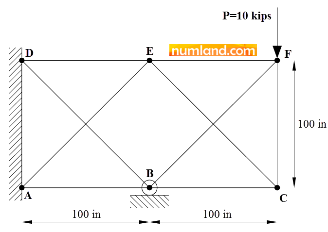
Consider the truss shown in the Figure including 9 members, which can rotate freely at the joints. The whole system is constrained at two points of A and D and a roller support of B. The members CE and BF as well as AE and BD do not intersect each other, so, there is no joint in the middle of these members. Because of manufacturing error, CF is 0.1 in shorter than the length of 100 in (99.9 in). Accordingly, there might be a pre-load in this member as well as the others related to this one. In addition, a concentrated force of 10000 lb, symbolized by P, is applied on the point F. The point of B has been pulled down 0.05 in and kept ny the support. The entire system is, also, heated in order to increase the temperature 50 oF. It causes thermal stresses in all members. This Tutorial leads you through the Abaqus\CAE modeling process to look for the stress in CF member and reaction force in the point B. More is, the results will be compared with the reference [1]. All lengths are in inch and all members cross-sectional areas are 3.33333 in2. The members are made from steel with the modulus of elasticity of 30×106 psi and thermal expansion coefficient of ![]() .
.
Creating the model:
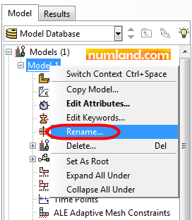
First of all, rename the Model-1 to 2D truss, considering Figure 2.
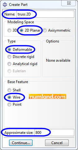
Click on icon ![]() (Create Part) and choose the items of opened window as shown in Figure 3. To explain more, the evaluated truss can be defined in 2D space so in the section of Modeling Space select the item of 2D. Every truss member behaves like a wire, so that, Base Feature of the part has been selected Wire. Moreover, Approximate size specifies dimension of sketching area. To show the model entirely this parameter is normally considered 4 times bigger than the maximum length of the structure. For this reason, the length of 800 has been selected. Press Continue and go to the next step.
(Create Part) and choose the items of opened window as shown in Figure 3. To explain more, the evaluated truss can be defined in 2D space so in the section of Modeling Space select the item of 2D. Every truss member behaves like a wire, so that, Base Feature of the part has been selected Wire. Moreover, Approximate size specifies dimension of sketching area. To show the model entirely this parameter is normally considered 4 times bigger than the maximum length of the structure. For this reason, the length of 800 has been selected. Press Continue and go to the next step.
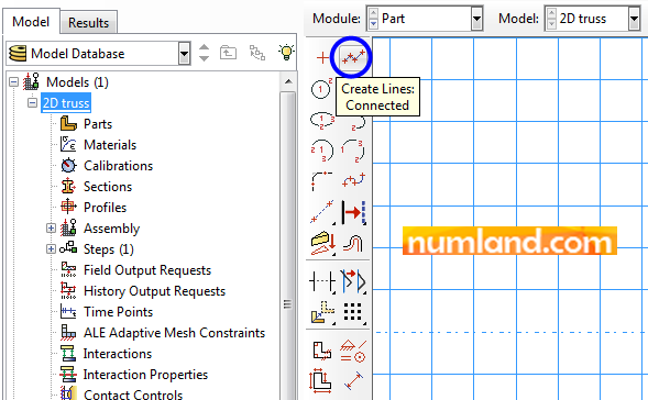
To start drawing the sketch, as shown in Figure 4, select the icon ![]() (Create Lines: Connected).
(Create Lines: Connected).
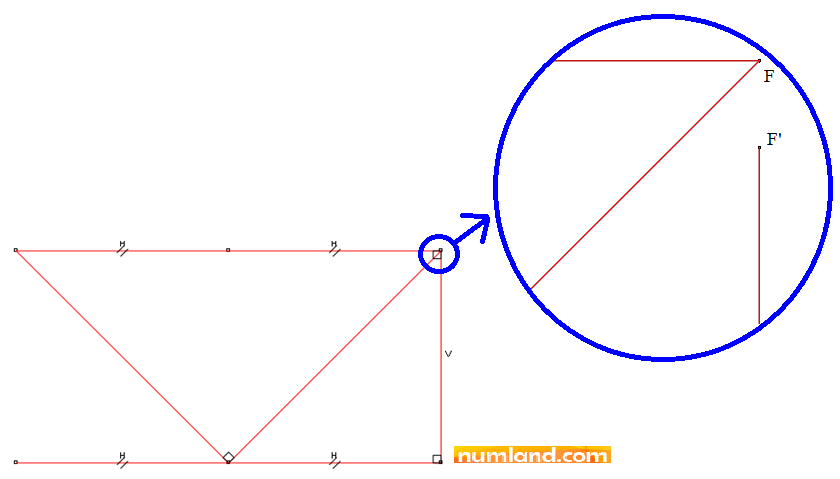
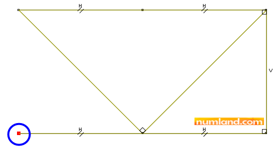
The geometry of truss must be created in two steps because one of its members (CF) is shorter than 100 in. The first step includes drawing 3 members of AB, BC and CF’. So, in prompt area, insert the coordinates given in Table 1 with the sequence of A > B > C > F’. You can press Enter key to confirm the coordinates each. Finally, press Esc to finish the first step. Note that the point F’ has a distance of 0.1 in with the point F.
Table 1: The coordinates needed for drawing AB, BC and CF’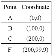
After doing this, you will see Figure 5 in viewport.
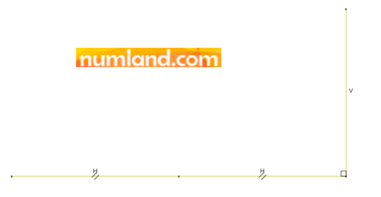
Again, click on icon ![]() (Create Lines: Connected) and use coordinates in table 2 to draw remained members. Consider the order of inserting points as given in the table.
(Create Lines: Connected) and use coordinates in table 2 to draw remained members. Consider the order of inserting points as given in the table.
Table 2: Coordinates used for creating remained members in the second step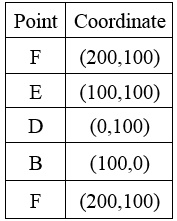
Use the icon ![]() (Auto-Fit View) to see the whole of sketch drawn. Take notice that 2 truss members, which are AE and EC, have not been created in this stage, because in meshing step the intersection points will be considered as Nodes. Therefore, we will make these members in meshing steps by creating elements directly.
(Auto-Fit View) to see the whole of sketch drawn. Take notice that 2 truss members, which are AE and EC, have not been created in this stage, because in meshing step the intersection points will be considered as Nodes. Therefore, we will make these members in meshing steps by creating elements directly.
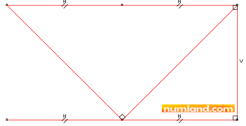
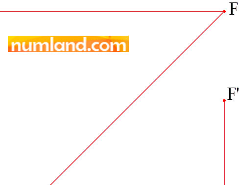
In order to observe shrinkage in CF the view has been zoomed in on points F and F’ which is displayed in Figure 7.
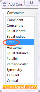
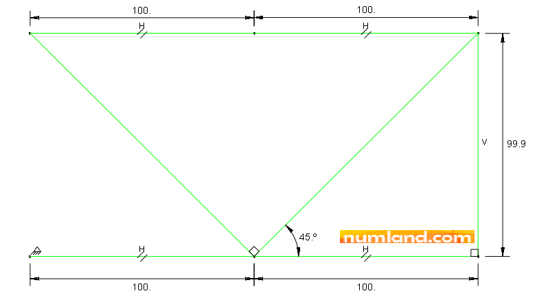
Note 1You would better to constrain the sketch you drew, to prevent it from moving during the modeling process. To do this click on icon
Select the point specified in Figure B and press Done in prompt area.
This causes to emerge a triangle shape symbol which indicates that this point has been fixed. To fix the lengths of members use the icon Doing the same, specify the lengths of other members shown in Figure C. To put dimension on the angle, select both sides of the angle one after another. The fully constrained structure will be indicated with Green color as you see in Figure C. If you put extra constraints the color will change to Pink which is unacceptable. In this kind of situation some constrains need to be omitted.
|
To exit from sketch environment click on Done button in Prompt Area. This shows the truss drawn in Viewport same as what you see in Figure 6.
Meshing the model:
Enter Mesh module and like Figure 31 in Tutorial 1, set to create 1 element on each member. Clicking on icon ![]() (Mesh Part) and selecting the option Yes, create meshes on the truss. As mentioned above, we need to create two remained members directly. So, before you change the type of elements to Truss Element, create these elements, considering Figures 8 to 11.
(Mesh Part) and selecting the option Yes, create meshes on the truss. As mentioned above, we need to create two remained members directly. So, before you change the type of elements to Truss Element, create these elements, considering Figures 8 to 11.
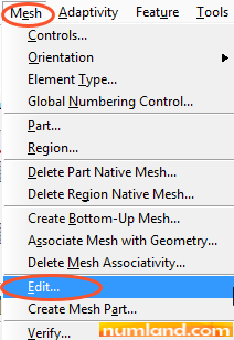
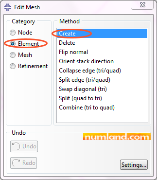
Select the items pointed out in Figure 9.
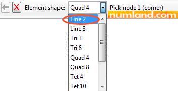
As truss elements in this case are linear having 2 nodes, select the item Line 2 in prompt area.
To make the first element, click on node 1, then node 2 which are pointed out in Figure 11. When doing this, notice the messages given in prompt area. Press OK button to confirm selecting two nodes. This creates the element of AE.
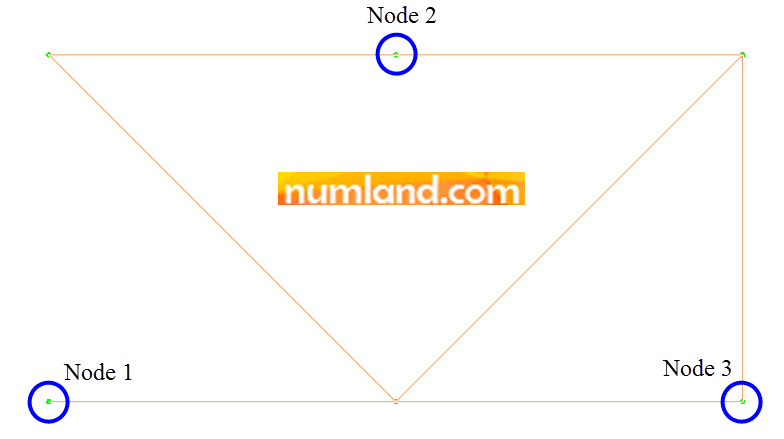
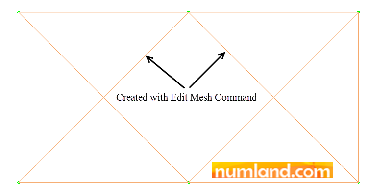
Do the same to create second element by clicking on nodes 2 and 3. Figure 12 depicts all components of the geometry of complete truss model. Notice the green points on the end points of each element, which are known as nodes. There is no node on intersected points of members we have just created. Finally, close the window Edit Mesh.
To change the elements type to Truss Elements click on the icon ![]() (Assign Element Type). As you see in Figure 13, unlike Tutorial 1, a message asks you to select the region that you want to assign element type to. The item geometry selects the elements that are meshed on a specific geometry which is made in Part module. The other item, orphan mesh, is for choosing the elements that have no geometry behind. Here, orphan meshes are the one we made by Edit Mesh tool. The imported meshes from the other software into the Abaqus are considered as orphan meshes too.
(Assign Element Type). As you see in Figure 13, unlike Tutorial 1, a message asks you to select the region that you want to assign element type to. The item geometry selects the elements that are meshed on a specific geometry which is made in Part module. The other item, orphan mesh, is for choosing the elements that have no geometry behind. Here, orphan meshes are the one we made by Edit Mesh tool. The imported meshes from the other software into the Abaqus are considered as orphan meshes too.

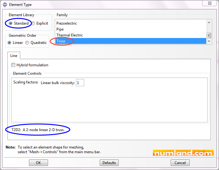
While the item geometry is selected drag all parts of the model. As you see the color of members that were created in Part module changes to the red. Press Done button, then select Truss item in opened window, shown in Figure 14, and, finally, press OK.
To assign truss type elements on members of AE and EC, do the same process but select orphan mesh in prompt area as selected region.

Defining Material properties:
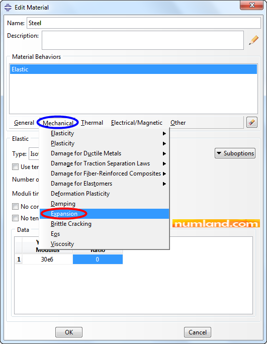
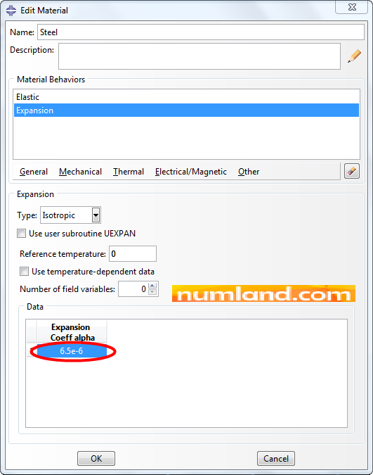
Enter Property module and going through the process explained in Figures 12 and 13 of Tutorial 1, create a material, named Steel, with Elasticity Modulus of 30×106 psi and Poisson’s Ratio of zero. Furthermore, in order to consider thermal stresses you need to define thermal expansion coefficient. To do this, as Figure 16 shows, select Expansion from Mechanical list, then insert the value of 6.5×10⁻⁶ in related box like Figure 17.
Clicking on OK completes defining the material with name of Steel.
Same as what explained in Figures 14 and 15 of Tutorial 1, clicking on icon ![]() (Create Section), create a truss type Section with cross-sectional area of 3.33333 in2.
(Create Section), create a truss type Section with cross-sectional area of 3.33333 in2.
To assign sections to the elements click on icon ![]() (Assign Section). A message in prompt area (see Figure 18) asks you to choose the region in which elements were made. The items Geometry and Mesh select the elements that are meshed on a specific geometry or made without any geometry, respectively.
(Assign Section). A message in prompt area (see Figure 18) asks you to choose the region in which elements were made. The items Geometry and Mesh select the elements that are meshed on a specific geometry or made without any geometry, respectively.

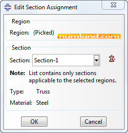
Same as the step that you assigned elements types in, you must assign the section on both geometry based elements (select Geometry) and directly created elements (select Mesh), separately. In both steps, as shown in Figure 19, select Section-1 and press OK. This causes that color of all elements, whether made on geometry or directly, changes to Cyan.
Assembling the truss in Assembly module:
Enter Assembly module and clicking on icon ![]() (Instance Part), insert the part into assembly environment. Note that in prior steps we meshed the part before putting it in the assembly environment, as a result, we face only Dependent (to the Part) option. In this step, considering the process explained in Figures 19 and 20 in Tutorial 1, save the model into a folder with name of 2D Truss.
(Instance Part), insert the part into assembly environment. Note that in prior steps we meshed the part before putting it in the assembly environment, as a result, we face only Dependent (to the Part) option. In this step, considering the process explained in Figures 19 and 20 in Tutorial 1, save the model into a folder with name of 2D Truss.
Defining the static analysis Steps:
Enter the Step module. Although you can solve this problem in one step, to comprehend the process of simulating tension caused by 0.1 in deviation in length of member CF, we separate this load condition and applying other forces. So, the first step includes connecting the points F and F’ to simulate tension. Then, we put the load of 10000 lb, thermal load and displacement in the point B in the second step.
Click on icon ![]() (Create Step) and select the items displayed in Figure 20, then, press Continue.
(Create Step) and select the items displayed in Figure 20, then, press Continue.
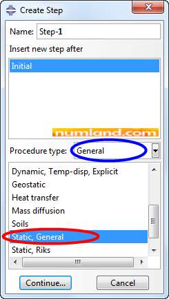
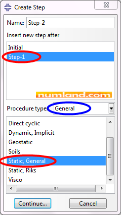
Accepting all conditions in Edit Step window, click on OK. This creates the first step which is Static. Again click on icon ![]() (Create Step) and choose the items shown in Figure 21. By doing this, the second step will be created after Step-1, named Step-2.
(Create Step) and choose the items shown in Figure 21. By doing this, the second step will be created after Step-1, named Step-2.
Same as previous step, accept all conditions brought in Edit Step window by clicking on OK.
Pre-tension in CF’ member (Putting the point F’ on F):
Enter Interaction module. In this area, first, we will create a Connector Section with type of Translator, then, we will make a connector between points of F’ and F and assign the Section.
Note 2Connector elements, which are meshless elements, are used for mechanically connecting two points of the model. For instance, various parts of seat belt or door hinges can be simulated by connectors. Every connector contains one wire which depends on Assembly, but it differs from wire in Part module as the connector elements cannot become discrete (meshed). To define features of connectors, it is needed to assign Sections containing local coordinate systems and if needed connectors properties. |
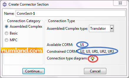
Click on icon ![]() (Create Connector Section) and select Translator as displayed in Figure 22, then, press Continue button.
(Create Connector Section) and select Translator as displayed in Figure 22, then, press Continue button.
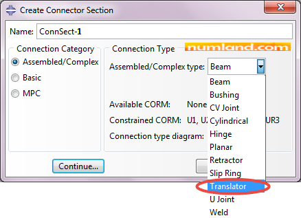
Note 3In Create Connection Section window, when Translator is selected as the Connection Type, U1 has been written next to the item Available CORM (Components of Relative Motion), which means throughout proportional degree of freedom, the U1 is the one which can be defined. Furthermore, the other degrees of freedom are constrained as mentioned by Constrained CORM: U2, U3, UR1, UR2, UR3.
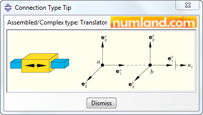
In order to see the schema of the connector click on icon
|
The aim of defining connector in this Tutorial is to bond two points of F and F’. Therefore, there is no need for specifying any feature for the connector. So, click on OK to close Edit Connector Section window. This makes a Connector Section with type of Translator.
To create a connector, first, zoom on the points using icon ![]() (Box Zoom View) shown in Figure 23.
(Box Zoom View) shown in Figure 23.

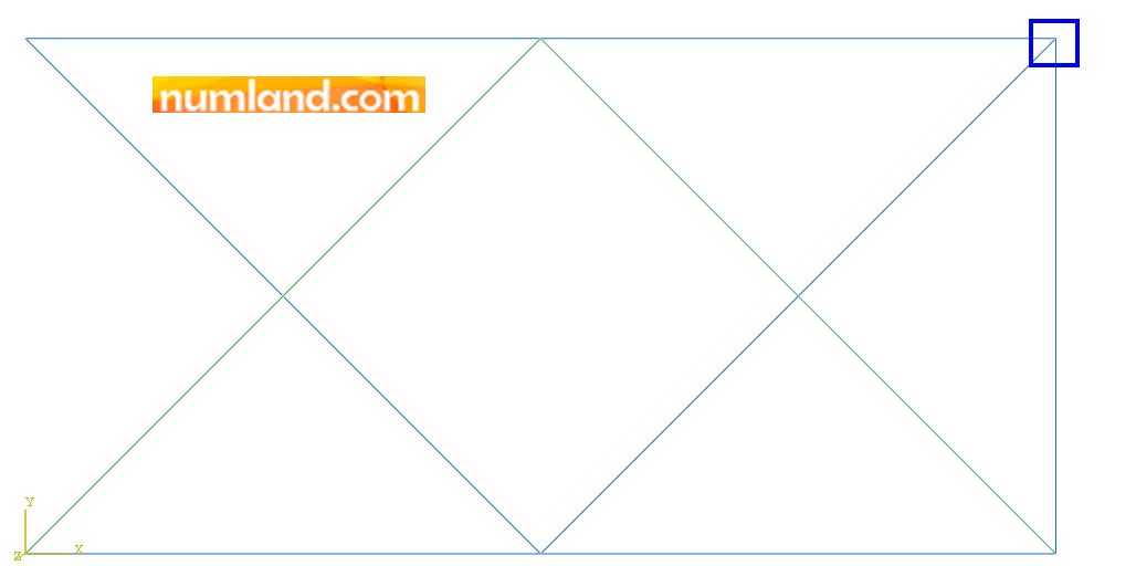
Drag the area displayed in Figure 24 and keep doing it until you see the points like what displayed in Figure 25.
In order to build the connector (wire), click on icon ![]() (Connector Builder). Select the points sequentially as you are asked in prompt area. This brings up a window with name of Connector Builder. As Figure 26 demonstrates, select the items and then press OK.
(Connector Builder). Select the points sequentially as you are asked in prompt area. This brings up a window with name of Connector Builder. As Figure 26 demonstrates, select the items and then press OK.
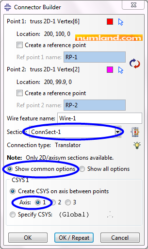
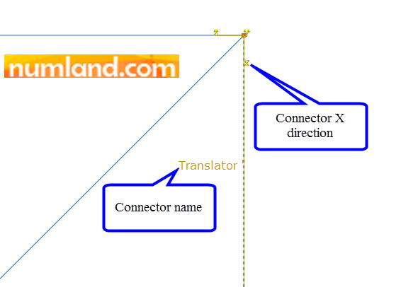
This makes a connector, with type of Translator, between two points of F and F’ as displayed in Figure 27.
Defining force type output for the Connector:
We are looking for the internal force in the member of CF. There exist two methods to obtain this value:
1- Same as what was done in the Tutorial 1, we can calculate the force by multiplying the stress in the element to its cross-sectional area
2- Defining output of force in the connector
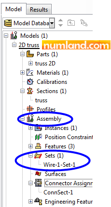
In this Tutorial we use the second method. In order to request the output of force in the connector, first, we need to use the Set which was created when we defined the connector.
Note 4Set in Abaqus, collects some items such as elements, nodes, points, edges, faces, solids, connectors, etc. or even their compounds together. This tool is used to facilitate selecting these specific items or to define a particular output on them. |
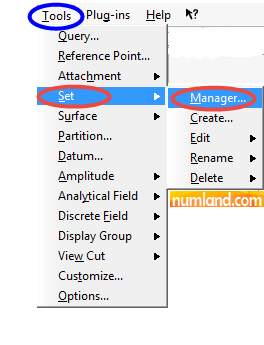
When defining connectors, Abaqus by default creates a Set and we do not need to do it again. Using the tool shown in Figure 28, you can see mentioned Set.
Note 5The Sets can be observed via the Model Tree too, as shown in Figure A. You can click right on each set to do what you aim. Note that using previous method which was opening Set Manager window only helps to access the Sets that are made in the module you run the command. There might be some extra Sets that are created while you were defining material properties in Property module. This has no effect on either modeling process or earned results.
|
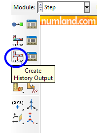
To define a specific output being obtained from connectors, go back to Step module and click on the icon of Create History Output which is pointed out in Figure 29.
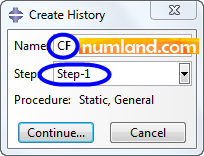
Configure the opened window same as what Figure 30 illustrates then press Continue.
After this, the window of Edit History Output Request comes up. Select the items same as what displayed in Figure 31. Choose Set of Wire-1-Set-1 as Domain. Moreover, in the section of Output Variables select Connector > CTF > Total forces and moments and CTF1 (force in direction of 1), respectively. Note that the Translator type connector can only evaluate the axial direction symbolized by 1. Click on OK to confirm and close the window.
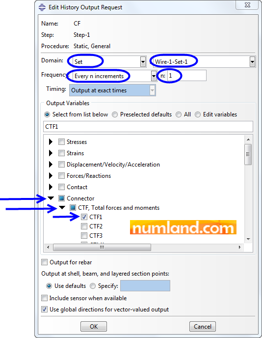
Note 6In Edit History Output Request window, the item of Frequency is put on the option of Every n increments which means that after every n increment, 1 output will be written in the results file. Here, the value of n is considered 1. This causes that all outputs in all increments will be recorded. |
Defining Boundary conditions and Loads:
In this step we are going to create the conditions mentioned below considering Figure 32:
1- The points A and D are constrained in vertical and horizontal orientations.
2- The member CF is tensioned as it is 0.1 in shorter than 100 in.
3- The point B moves down 0.05 in and stays at that position.
4- A force of 10000 lb, named P, is applied on the point F vertically.
5- The entire structure is heated with temperature change of 50 oF.

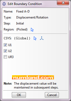
In order to fix the points of A and D, click on the icon ![]() (Create Boundary Condition); then, choose the items Figure 33 shows. Finally, press Continue.
(Create Boundary Condition); then, choose the items Figure 33 shows. Finally, press Continue.
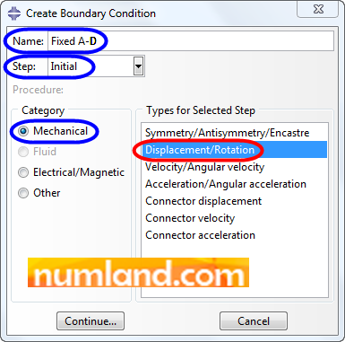
Note 7As constraining A and D exist before all other conditions, we need to select Initial as the step of applying it. This means the boundaries will have been constrained by the time steps at the beginning. However, it would not make difference if we defined it in Step-1. |
Select Geometry button in prompt area; then, select the points of A and D using Shift key. Finally, press Done. In opened window, which is Edit Boundary Condition, enable U1 and U2 and press OK. This constrains the points of A and D in vertical and horizontal directions.
To simulate the tension in the member of CF we need to put F on F’. So, create a displacement of -0.1 in the Translator connector defined in prior steps. Again, click on icon ![]() (Create Boundary Condition) but this time select Connector displacement as shown in Figure 34.
(Create Boundary Condition) but this time select Connector displacement as shown in Figure 34.
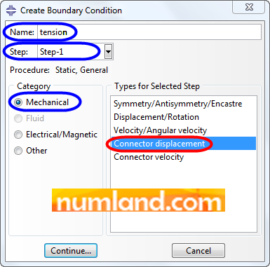
Note 8In the first step (Step-1), the points of F and F’ meet each other while they were separated in Initial step. After this step, nodes and elements of the structure will deform based on prevalence of tension in CF. That is the reason we made 2 steps as the first step involves modifying the initial geometry (Separated F and F’) to the real condition (Tension in CF). Obviously, the other boundary conditions and loads will be defined in Step-2. |
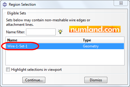
As Figure 35 and 36 display, select the Set of connector which was defined automatically, during creating the Translator Connector. To do this, first, disable Create set in prompt area and select Set button.

After this, select the Set with name of Wire-1-Set-1 in Region Selection window and Continue.
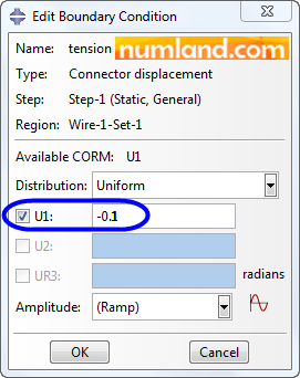
As you see in Figure 37, the only possible option in Edit Boundary Condition window related to the Translator Connector is U1, which is wise. So, enable this item and insert the value of -0.1, then, click on OK. The minus (-) sign means you make the two end points of the connector (with length of 0.1 in) move in regard to lay on each other. This is clarified by two orange arrows which appear on the connector.
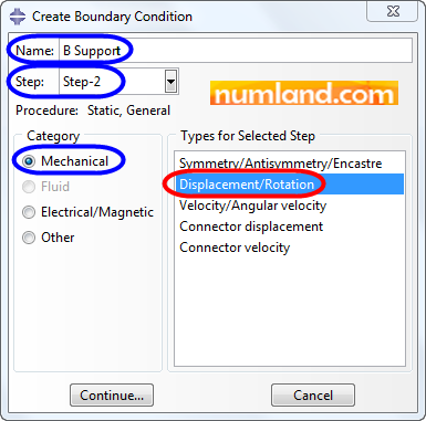
To displace the point B, 0.05 in, click on icon ![]() (Create Boundary Condition). Configure opened window same as the way Figure 38 shows and then Continue. Again, note that this condition is defined in Step-2.
(Create Boundary Condition). Configure opened window same as the way Figure 38 shows and then Continue. Again, note that this condition is defined in Step-2.
Selecting Geometry button in prompt area, pick the point B, then, click on Done in prompt area. As Figure 39 displays, insert the value of -0.05 next to U2 which symbolizes displacement along Y direction.
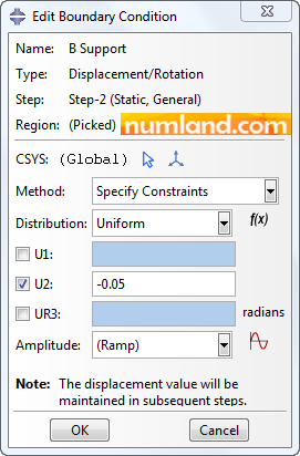
Press OK button. This leads to an orange arrow appears on the point B with direction to the bottom. To observe the boundary conditions defined, click on the icon shown in Figure 40.
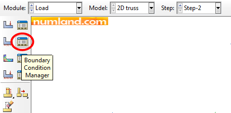
This brings up the Boundary Condition Manager window and the list of defined boundary conditions as you see in Figure 41.
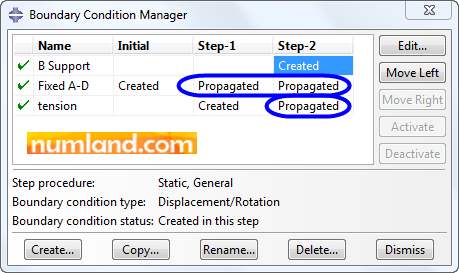
Note 9Take notice to the items of Created and Propagated. The first indicates the step in which the boundary condition is created. Propagated expression shows that the results of prior step will be transmitted to related step. For instance, tension in the member of CF, which is created in Step-1, will influence Step-2. In other words, its results will sustain in Step-2 as well. |
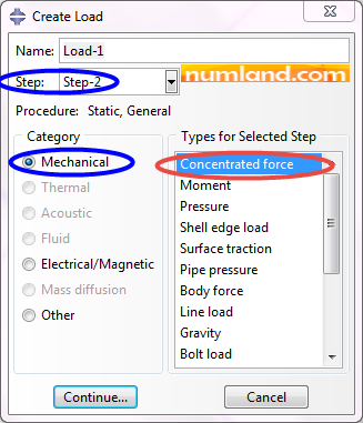
In order to apply the force of 10000 lb, click on the icon ![]() (Create Load) then set the items as demonstrated in Figure 42 and Continue. Note selecting Step-2 as the step of applying the force.
(Create Load) then set the items as demonstrated in Figure 42 and Continue. Note selecting Step-2 as the step of applying the force.
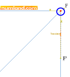
By using the icon ![]() (Box Zoom View) zoom on the point of F, then, select Geometry button in prompt area. As Figure 43 displays choose the point F and complete the process by pressing Done.
(Box Zoom View) zoom on the point of F, then, select Geometry button in prompt area. As Figure 43 displays choose the point F and complete the process by pressing Done.
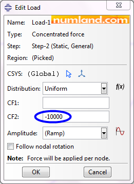
Configure the Edit Load window as shown in Figure 44, then, press OK. Notice the arrow appeared on the point F which shows the orientation of demanded force.
In the way you observed list of boundary conditions, you can see the ones for Loads by clicking on the icon ![]() (Load Manager) which is next to the icon
(Load Manager) which is next to the icon ![]() (Create Load). Notice the step in which the load is applied.
(Create Load). Notice the step in which the load is applied.
In order to apply thermal load on the elements click on icon ![]() (Create Predefined Field), then, select Temperature as shown in Figure 45, and finally, press Continue.
(Create Predefined Field), then, select Temperature as shown in Figure 45, and finally, press Continue.
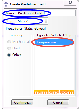
Select Geometry option in prompt area and then drag all truss members.
Note 10By selecting the item of Geometry in prompt area, you can only select the members that are created in Part module. There is only one element on each truss member, so that each member has 2 nodes on its end points. Same as displacement, temperature will be defined on nodes and this means while we are selecting Geometry and then all of the structure, temperature increase will occur on all joints of truss. Therefore, there is no necessity to select the elements made in Mesh module. Note that although in this step we selected all parts, temperature increase would only apply on nodes not elements. |
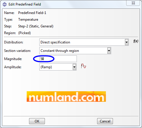
Increase the temperature 50 oF as displayed in Figure 46, then, press OK. There emerge some yellow squares on elements showing temperature change has been applied.
Analyzing the problem:
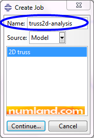
Enter Job module and click on icon ![]() (Create Job). Name the job truss2d-analysis as shown in Figure 47 then Continue.
(Create Job). Name the job truss2d-analysis as shown in Figure 47 then Continue.
To remind the rules for naming a job refer to Note 7 in Tutorial 1. Analyze the structure using the procedure illustrated in Tutorial 1, Figure 34. After the job finished, in Job Manager window, click on Monitor button to observe information of solving process. As shown in Figure 48, section 1, both steps have been done completely, in 1 increment. In the next step, select Warnings tab.
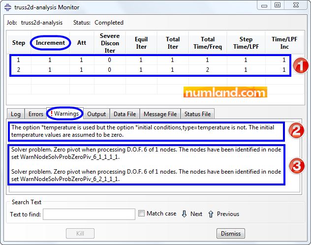
Section 2 in Figure 48 points out the message saying: there is no definition for the initial temperature of the model and it has been assumed to be zero, which is what we want. So, this warning is negligible.
It is said in section 3 that the Abaqus Solver faced a problem related to 6th degree of freedom of a node.
Note 11Each node, generally, has 6 degrees of freedom. In Abaqus, they are known with a number from 1 to 6 as following:
In case the problem can be evaluated in 2D spaces, the nodes only have maximum 3 DOF which are 1st, 2nd and 6th degrees of freedom. That is the reason when Boundary Condition is being defined, these degrees of freedom are available as shown in Figure B.
|
This warning appears when the model defined is over-constrained. It means the number of equations derived from FEM (forces, constraints and boundary conditions) exceeded the number of unknown values. Based on the problem, this event may cause wrong results. Therefore, as a professional Abaqus user, we need to investigate why 6th DOF of 2 nodes has become zero pivot (In lessons of FEM in MATLAB, we will describe the word Pivot through solving a problem by Gaussian elimination method).
When it comes to the problems that can be evaluated in 2D space, same as the one we are working on, there are only U1 and U2 as the degrees of freedom defined on nodes of truss elements. However, the Translator Connector has all possible 3 DOF (U1, U2, UR3) considering that 2 of them (U2 and UR3) are constrained. Here U1 and U2 of translator connector can be projected on U1 and U2 of truss elements, while UR3 of both nodes of translator connector being constrained will generate 2 extra equations, which results that the model becomes over-constrained. In order to deal with this issue and not having mentioned warning, we must have used Axial Connector, but here using Translator Connector works and earns correct answers too. In Tutorial 3, using Axial Connector will be considered and explained though.
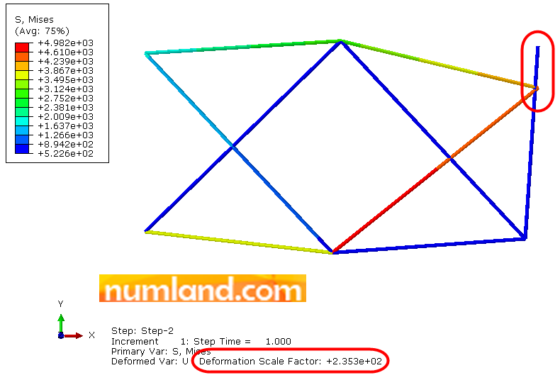
After all, to see the results enter Visualization module, then, click on icon ![]() (Plot Contours on Deformed Shape). This gives deformed shape of the model affected by the loads. As shown in Figure 49, points of F and F’ seem to be departed while we made them connected using translator connector. The reason is Abaqus represents the deformed shape with Scale Factor.
(Plot Contours on Deformed Shape). This gives deformed shape of the model affected by the loads. As shown in Figure 49, points of F and F’ seem to be departed while we made them connected using translator connector. The reason is Abaqus represents the deformed shape with Scale Factor.
| Note 12
Deformation Scale Factor is a tool to multiply the displacements of nodes in order to ease observing the model. This scale is pointed out in Figure 49 which is specified automatically. However, you can change it from Options > Common > Basic > Deformation Scale Factor in menu bar. |
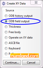
To validate whether F and F’ laid on each other or not, you can consider their displacements in X and Y directions and see if they make sense. For doing this, click on the icon ![]() (Create XY Data) and select the item displayed in Figure 50, then, Continue. This item allows you to pick the results from viewport directly.
(Create XY Data) and select the item displayed in Figure 50, then, Continue. This item allows you to pick the results from viewport directly.
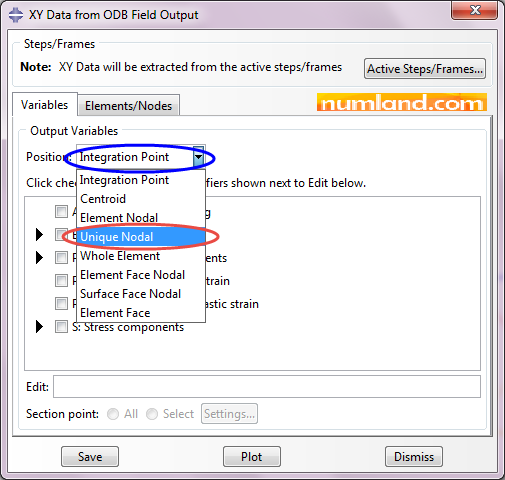
Same as Figure 51, select the item Unique Nodal which is for getting the results from Nodes.
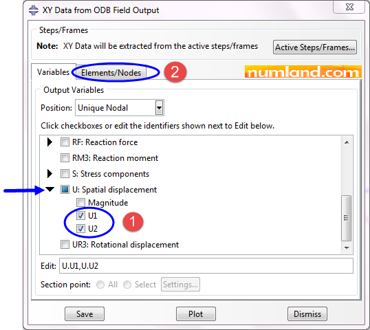
After this, select the displacements U1 and U2 as you see in Figure 52, then, got to Elements/Nodes tab to select the nodes in viewport.
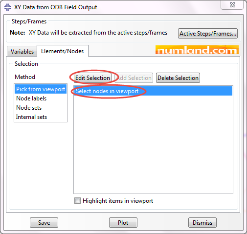
As shown in Figure 53, click on Edit Selection and using Shift key, select the points displayed in Figure 54, then, press Done button.
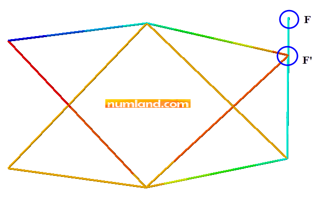
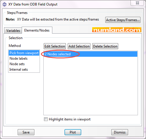
You will see 2 Nodes selected in window of XY Data from ODB Field Output as displayed in Figure 55.
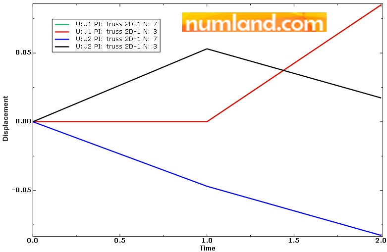
We are doing this to validate if the connector worked correctly, so that there is no need to Save the data. Just click on Plot button to see the way these displacement values changed during the steps (time). Figure 56 shows the related graphs. U1 of both nodes behaved exactly the same and this is the reason we have 3 lines rather than 4. Once you plot the values, they will be saved in memory temporarily as we will use them in the next step.
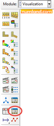
Now, click on the icon ![]() (XY Data Manager) which is specified in Figure 57 to see magnitudes of displacements in digit. Note that there can be observed the output values that you plotted in previous step.
(XY Data Manager) which is specified in Figure 57 to see magnitudes of displacements in digit. Note that there can be observed the output values that you plotted in previous step.
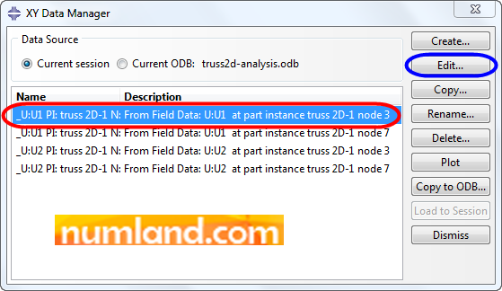
In opened window, select the displacement item shown in Figure 58 and press Edit button. This belongs to U1 of node 3 (Point F’).
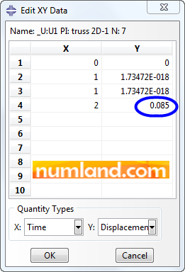
The final displacement of node 3 in X directions has been pointed out in Figure 59.
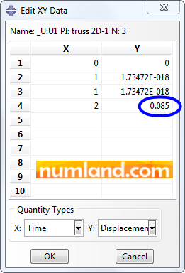
There exist 4 rows of numbers in Edit XY Data window. Remember we analyzed the problem in 2 steps which were solved in 1 increment each. The first row is related to the Initial step where no displacement exists. The second though is resulted from Step-1 as we have a tinny displacement in X direction. This is assumed as the initial inputs of Step-2 which is recorded in third row. The last one is the displacement of node 3, in X direction, when all loads are applied on the structure. This is the result of Step-2. Write this magnitude down to compare it with the one of node 7 (Point F). Do the same process for the node 7 as illustrated in Figure 60.
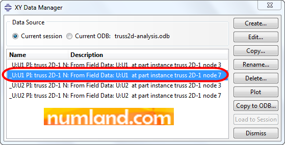
As you observe in Figure 61, the U1 magnitude of node 7 is same as the node 3 in all steps which means both of them displaced in X direction similarly.
Now see displacements in Y direction. Figure 62 shows how they changed over the steps.
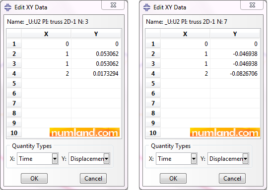
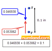
Considering initial 0.1 in distance between these two points, the Step-1 was supposed to make them lay on each other using the Translator Connector with displacement of -0.1. So, if you imagine this process, noticing displacement magnitudes in the second rows and the schema presented in Figure 63, you will learn that both points moved to cover the distance up.
In Step-2 which is the final step, both points (F and F’) must stay at the same position again. In other words, they must have moved together with the equal magnitude. It means that the connection created in Step-1 is maintained in second step as we anticipate. To find the displacement in Step-2, subtract displacement resulted in Step-1 from the one in Step-2 as following:
U2 (F) = -0.0826706 – (-0.046938) = -0.0357326
U2 (F’) = 0.0173294 – 0.053062= -0.0357326
As you see, displacements of two nodes in Step-2 are equal which means the connector worked properly.
After all, we compare the force created in member CF and the reaction force of the support B with reference [1]. First, click on icon ![]() (Plot Contours on Deformed Shape) in order to show the structure. In this Tutorial we will use a different method to Figure out the forces than the one in Tutorial 1. Click on icon
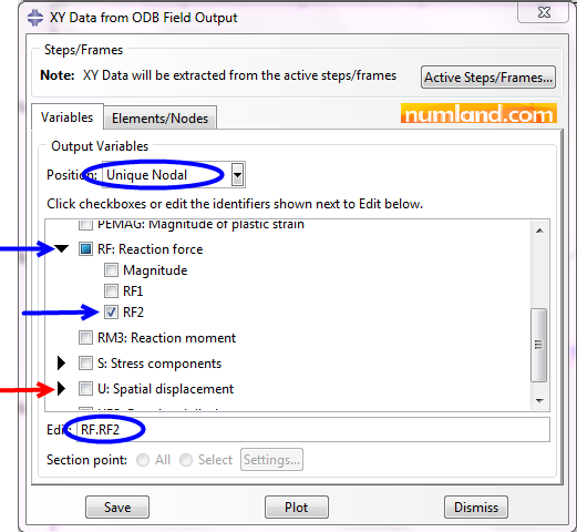
(Plot Contours on Deformed Shape) in order to show the structure. In this Tutorial we will use a different method to Figure out the forces than the one in Tutorial 1. Click on icon ![]() (Create XY Data) again. While the item ODB field output is selected press Continue. In opened windows, select the items displayed in Figure 64. Remember to disable Spatial displacement as we enabled it before. Doing this, RF.RF2 must be written in the edit box. Note we can probe reaction forces into nodes that we defined boundary conditions.
(Create XY Data) again. While the item ODB field output is selected press Continue. In opened windows, select the items displayed in Figure 64. Remember to disable Spatial displacement as we enabled it before. Doing this, RF.RF2 must be written in the edit box. Note we can probe reaction forces into nodes that we defined boundary conditions.
Click on the tab Elements/Nodes then select Edit Selection button. Select the point B and click on Done in prompt area. Now Plot the data as we did before. Next, click on icon ![]() (XY Data Manager) and then select Edit button. Figure 65 shows all forces magnitudes in all steps.
(XY Data Manager) and then select Edit button. Figure 65 shows all forces magnitudes in all steps.
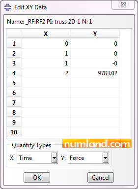
As you see, before Step-2 this force is sustained zero which means there was no force in Step-1 but it followed by a rise in Step-2 to 9783.02 lb when loads were applied on the structure. The magnitude is positive which means this force is in positive direction of Y. Table 3 presents this value and the one mentioned in reference [1]. They are close but actually, reference [1] has calculated the answer inaccurately. Though, if we use Castigliano’s method the precise answer will be obtained which is exactly equal to the answer Abaqus gave us.
In order to check the force in the member CF, click on icon ![]() (Plot Contours on Deformed Shape) again. Then, Click on icon
(Plot Contours on Deformed Shape) again. Then, Click on icon ![]() (Create XY Data), select ODB field output and Continue. Disable the item of reaction force (RF2), shown in Figure 66.
(Create XY Data), select ODB field output and Continue. Disable the item of reaction force (RF2), shown in Figure 66.
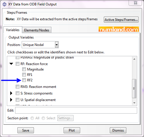
In window of XY Data from ODB Field Output, find S: Stress components as pointed out in Figure 67 and select S11. The item Centroid measure the stress in mid-point of elements. Remember that stress in whole length of the truss elements is equal.
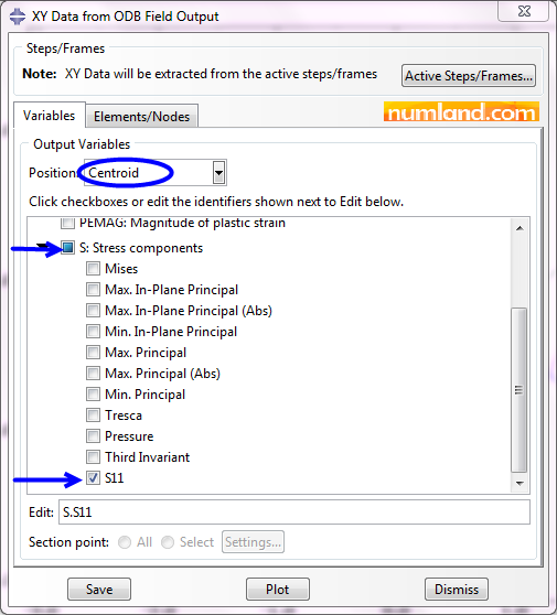
Go to tab Elements/Nodes, then, press Edit Selection button. In viewport, select the element of CF member and click on Done button. Press Plot to draw the graph of changing selected stress along the time. The graph demonstrates that there is an increase in the stress, as a result of tension in CF during Step-1. After that, because we applied a force of 10000 lb and other types of loads, this was followed by a drop. Now, click on icon ![]() (XY Data Manager) to see magnitudes of the mentioned stress which is presented in Figure 68.
(XY Data Manager) to see magnitudes of the mentioned stress which is presented in Figure 68.
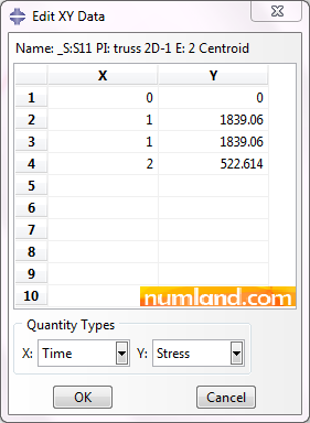
As we are looking for the force when whole loads are applied, the number reported in 4th row (Result of Step-2) is our answer. Multiply this number by the cross-sectional area of the member which was 3.33333 in2 to achieve the force in the member.
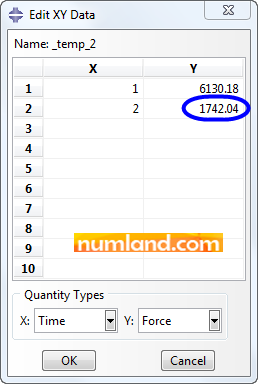
FCF = SCF × A = 522.614 × 3.33333 = 1742.045 lbs
This has been compared with the force brought in reference [1] through table 3. “+” symbol shows that the member CF is under the tension. This force, when there is no other load but tension, (result of Step-1) equals to +6129.59 lbs. This means tension has been decreased due to the loads we applied in Step-2.
Table 3: Results of Abaqus and Reference [1] ![Results of Abaqus and Reference [1]](https://www.numland.com/wp-content/uploads/01 Courses/001/1/01/00110102/00110102_T03ryF.png)
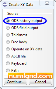
To get the force in connector, which is equal to the force in the member CF, click on icon ![]() (Create XY Data), then, like Figure 69, select the item ODB history output. Finally, press the Continue button.
(Create XY Data), then, like Figure 69, select the item ODB history output. Finally, press the Continue button.
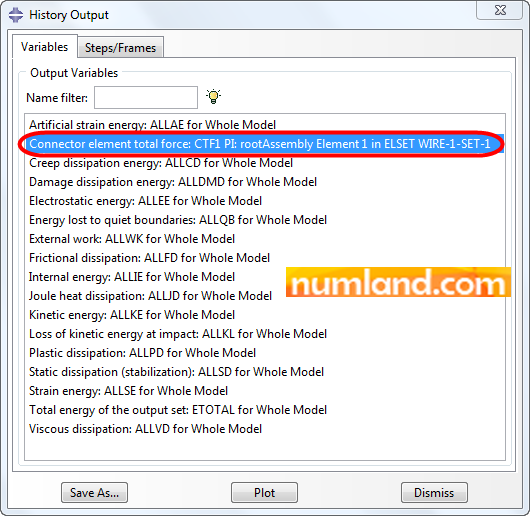
After that, the related window comes up, then, select the item shown in Figure 70. Finally, press the Plot button.
In the way you learned above, find the magnitudes of plotted outputs. They have been presented in Figure 71. As seen the internal force produced after Step-2 is exactly equal to the one we calculated from multiplying the stress to cross-sectional area of the element.
Reference:
[1] Timoshenko, S. P. and Young, D. H. “Theory of Structures,” end Ed., McGraw-Hill, New York, 1965, pp. 313-315.


Be the First to Comment!